using Pkg
Pkg.activate(".")5 Symbolic Regression
More details, we refer to MilesCranmer/SymbolicRegression.jl: Distributed High-Performance Symbolic Regression in Julia
Symbolic Regression (SR) is a type of regression analysis that searches the space of mathematical expressions to find the model that best fits a given dataset in terms of accuracy and simplicity. It utilizes binary trees to represent a function, and does not rely on a particular model as a starting point to the algorithm. Instead, initial expressions are formed by randomly combining mathematical building blocks such as - binary mathematical operators: \(+, -, *, /\); - unary analytic functions: \(\sin, \cos, \exp , \tanh, \dots\); - constants; - state variables.
Usually, a subset of these primitives will be specified by the person operating it, but that’s not a requirement of the technique. SR uses genetic programming, as well as more recently methods utilizing Bayesian methods and physics inspired AI to discover the equations. More details and benchmarks on symbolic regression methods can be seen in cavalab/srbench: A living benchmark framework for symbolic regression.
For example, we generate data from the following function which can be used to investigate the mass media impact on infectious disease: \[ f(I) = \beta \exp(-\delta I)I,\] and the binary tree of the equation is shown in 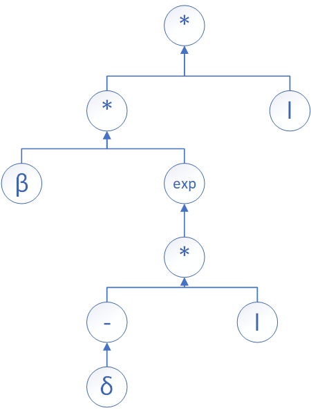
The function can be discovered by using symbolic regression, where the codes implemented in Julia are as following.
5.1 IMPORTANT: Activate Julia environment first
# Load packages
using SymbolicRegression
using SymbolicUtils
# Generating test data
I = collect(0:0.1:10)
f(x) = 0.2exp(-0.1*x)*x
Y = f.(I)


# choosing operations
options = SymbolicRegression.Options(
    binary_operators=(+, *, -),
    unary_operators=(exp,),
    npopulations=20
)


# equations searching
hallOfFame = EquationSearch(I', Y, niterations=150, options=options, parallelism=:multithreading
)
# output
dominating = calculate_pareto_frontier(I, Y, hallOfFame, options)
eqn = node_to_symbolic(dominating[end].tree, options)
(x1 * exp(-0.8866729615216796 - ((x1 - 5.823564614359717) * 0.10000000003526198))) * 0.271139613364567165.2 Project: predicting the peak time
Some immature ideas (may be wrong): - In Lectures 1&2 note, we know that \[I(t_p)=I_0+S_0\left(1-\frac{1}{\mathcal{R}_0}-\frac{\ln\mathcal{R}_0}{\mathcal{R}_0}\right),\] which implies the peak time \[t_p=f(\mathcal{R}_0).\]
Q: Can we use symbolic regression to search \(f\)?
- For real case data, you can learn \(\beta(t)=\mathrm{NeuralNetwork}(t)\) first \[ \left\{ \begin{aligned} & \frac{\mathrm{d}S}{\mathrm{dt}} = - \mathrm{NeuralNetwork}(t) S I, \\ & \frac{\mathrm{d}I}{\mathrm{dt}} = \mathrm{NeuralNetwork}(t) S I- \gamma I, \end{aligned} \right. \] then you get a new ODE. Solving this new ODE and setting \(\mathrm{NeuralNetwork}(t) S(t) I(t)- \gamma I(t)=0\), you can solve the peak time \(t_p\), and check whether \(t_p\) is minimum or maximum by checking the sign \[\frac{\mathrm{d}^2 I}{\mathrm{dt}^2}=(\mathrm{NeuralNetwork}(t) S I- \gamma I)'=(\mathrm{NeuralNetwork}(t)' S + \mathrm{NeuralNetwork}(t) S')I +(\mathrm{NeuralNetwork}(t) S - \gamma)I'.\]
Q: - How to solve this fixed point problem \(\mathrm{NeuralNetwork}(t) S(t) I(t)- \gamma I(t)=0\)? - How to improve the generalization (prediction ability) of the neural network embedded in differential equations? - How to combine these two ideas?